4.3.3.1. Predefined functions

In this section other possible data operations are shown, those are some predefined mathematical functions like inverse, square, square root, logarithm and average. In the last, the user must indicate the number of values to consider for calculating the average.

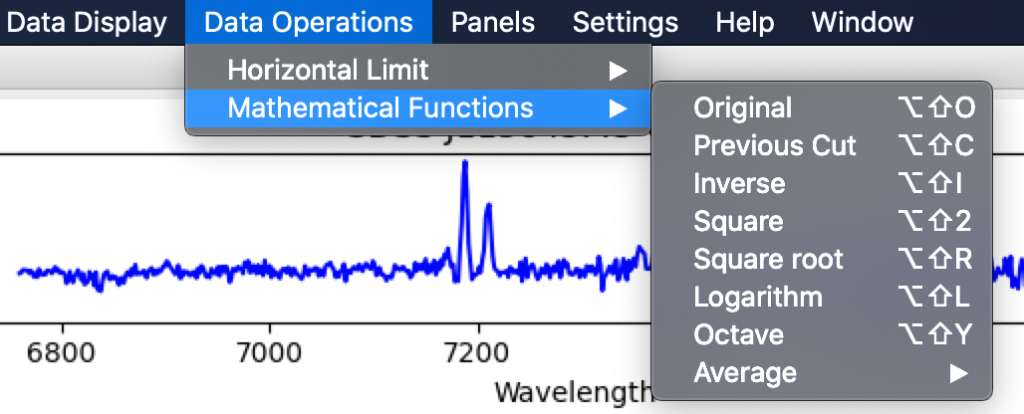
There are two ways to access the mathematical functions, one is with the mathematical functions item from the data operations menu (Image 51), which have the functions items; the other way is with the sliders and mathematical functions item from the data operation sub-menu in the panels menu (Image 48).

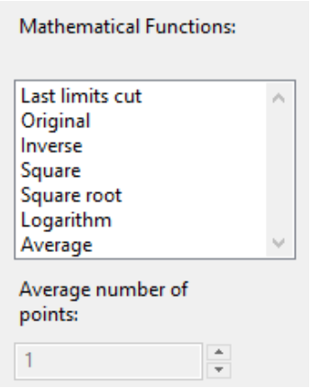
*Image 51 – Shows the mathematical functions sub-menu of the data operation menu, with its six items of the predefined functions.*

The items on the sub-menu mathematical functions and the items from the mathematical functions list on the sonoUno framework (Image 52) do the action when each one is pressed. The average item enables the number of points in the text box to select the number of values to be considered on the average calculus, by default is 1.

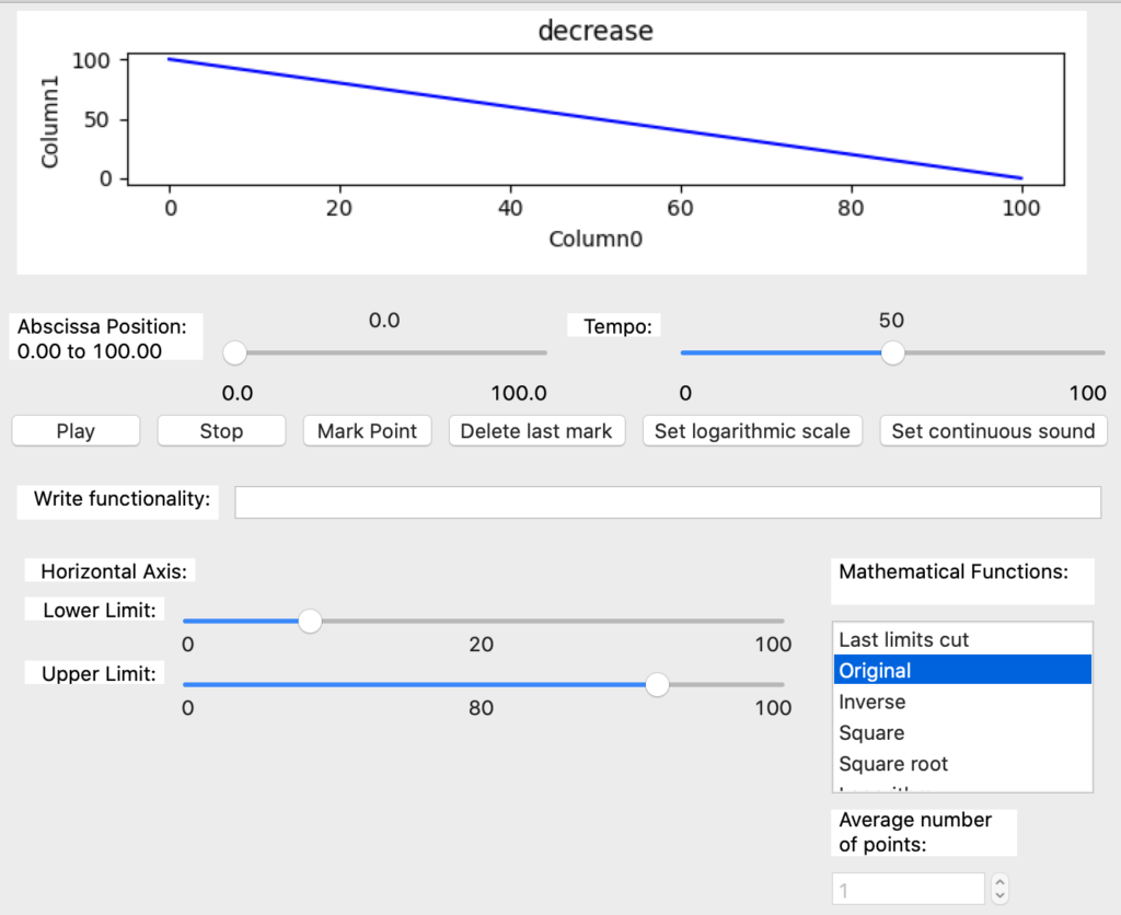
Image 52 – Shows the list of predefined mathematical function, are the same of the previous image. The text box of the bottom will be enabled with the average function and allow to set the number of points.

Coming up next, the mathematical functions are applied to a decreasing function with 100 values. The example starts with the decreasing function, lower limit set to 20 and upper limit set to 80.

The functionality named ‘Original’ allows to restore the plot to the original data without modifying the cut limit sliders. It’s useful for display the original data (Image 53).

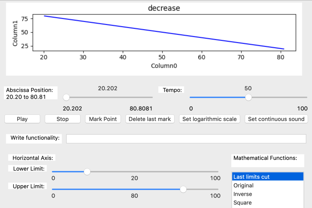
*Image 53 – The original function is selected; the cut limit sliders remains on the same position but the limits of the data on the reproduction and plot are the original.*

The functionality named ‘Last limit cut’ is to recover the last cut limits values set by the user (Image 54). When pressed after the ‘Original’ function, the plot is redrawn with the previous upper and lower limits. For example the upper limit is 80 and the lower limit is 20. Is useful to alternate with the original function, the user must have in mind that it is not possible to restore a previous cut value after changing a cut slider.

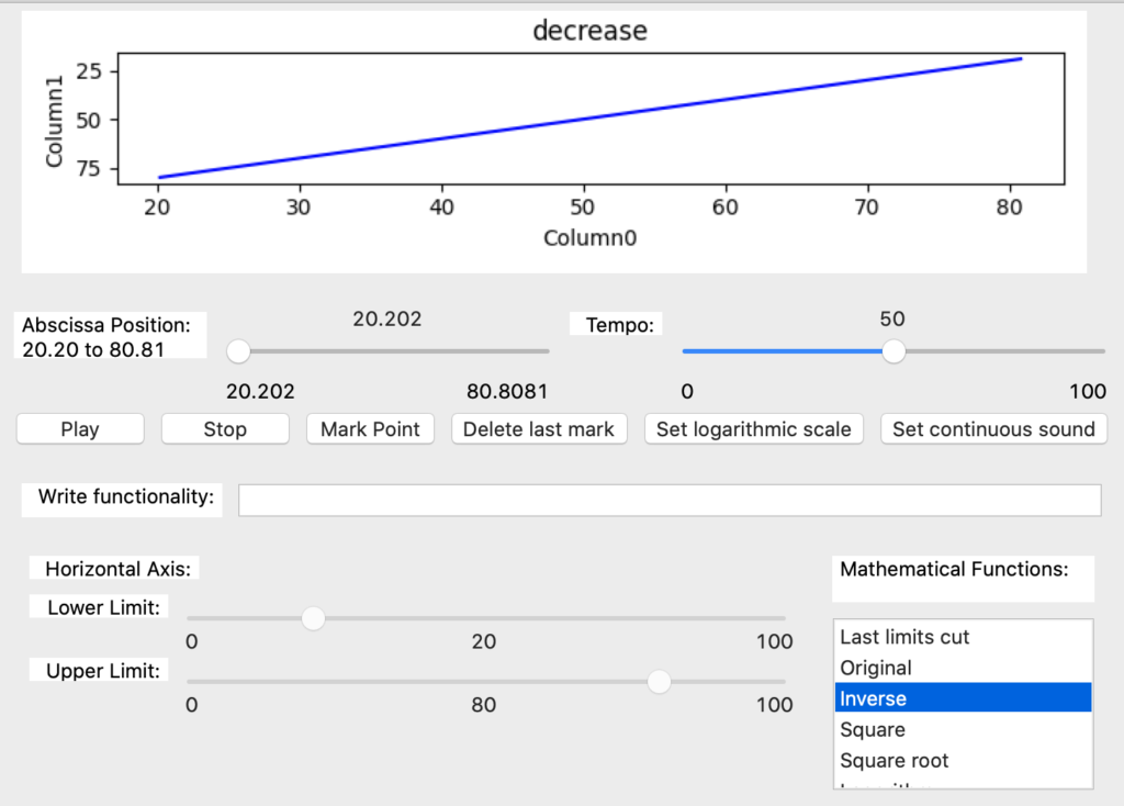
*Image 54 – The last limits cut is selected, the data for the reproduction and the plot have the same limits of the cut sliders again.*

The inverse function reverses the ends of the y axis (Image 55). It’s noticed that all the mathematical functions are calculated based on the original data and do not allow to cut the x axis.

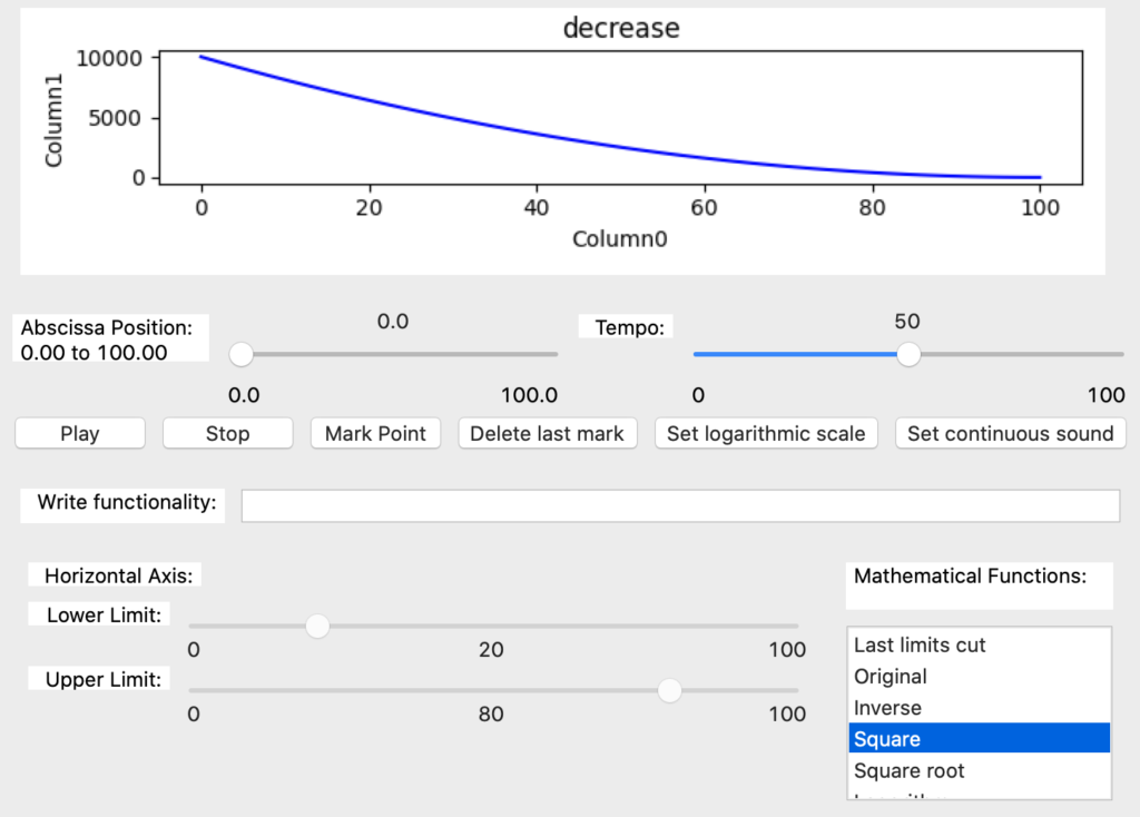
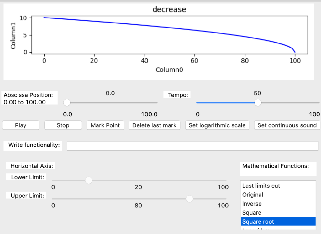
*Image 55 – The inverse function is selected; the data has been reversed with respect to the ordinate axis.*

The two next functions perform the square (Image 56) and square root (Image 57) to the original data.

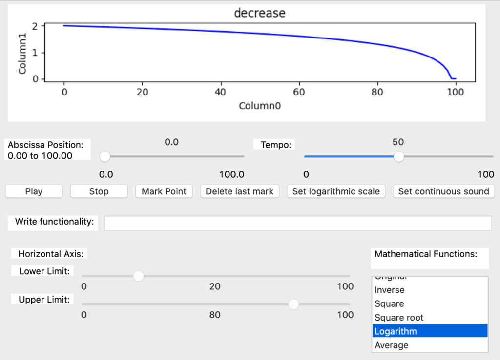
*Image 56 – The square function is selected. The image shows the square of the decreasing function.*

*Image 57 – The square root function is selected. The image shows the square root of the decreasing function.*

The logarithm item applies this function to the original data (Image 58).

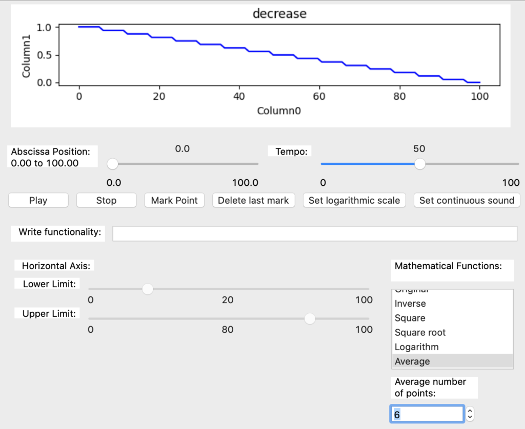
*Image 58 – The logarithm function is selected. The plot shows the logarithm of the decreasing function.*

Finally, the average function uses the number of points entered by the user to group the data and calculate the average on the original data. In the example the number of points is six (Image 59).

*Image 59 – The average function is selected. The text box under the mathematical functions list is enabled. In the image the number of points to set the average are six.*

Back to Index

Back to Home